library(tidyverse)
theme_set(theme_bw())

library(tidymodels)  # parsnip + other tidymodels packages

# Helper packages
library(readr)       # for importing data
library(broom.mixed) # for tidying Bayesian model output
library(dotwhisker)  # for visualizing regression results
library(skimr) # for variable summariesML Workflow with tidymodels
1 Libraries
In this article we use the tidymodels ecosystem to illustrate a complete machine learning workflow in a tidy, coherent, and reproducible manner.
Throughout the article, we revisit the fundamental components of the ML workflow:
- Data split
- Feature engineering
- Model building
- Model fitting
- Model prediction
- Model evaluation
We begin with the most basic workflow and later extend it using the recipe framework for more advanced preprocessing.
The material in this article is based on the case study provided at: https://www.tidymodels.org/start/case-study/. All exercises use the dataset included in that example.
The following packages are required:
2 Basic Model Building and Fitting
In the first case, we will focus on three steps:
- Exploring the data – Understanding the structure, distributions, and relationships within the dataset to inform subsequent modeling decisions.
- Specifying a model – Selecting an appropriate algorithm and defining its parameters based on the task and data characteristics.
- Fitting the model to the data – Training the model using the available data to estimate its parameters and capture underlying patterns.
2.1 Data
In this exercise we explore the relationship between:
- the outcome variable: sea urchin width
- feature 1: initial volume (continuous)
- feature 2: food regime (categorical)
A basic model for these variables can be written as:
width ~ initial_volume * food_regime## Data import ----------
df_Urchins <-
read_csv("https://tidymodels.org/start/models/urchins.csv") |>
setNames(c("food_regime", "initial_volume", "width")) |>
mutate(food_regime = factor(food_regime, levels = c("Initial", "Low", "High")))
## Explore the relationships ----------
ggplot(df_Urchins,
aes(x = initial_volume,
y = width,
group = food_regime,
col = food_regime)) +
geom_point() +
geom_smooth(method = lm, se = FALSE) +
scale_color_viridis_d(option = "plasma", end = .7)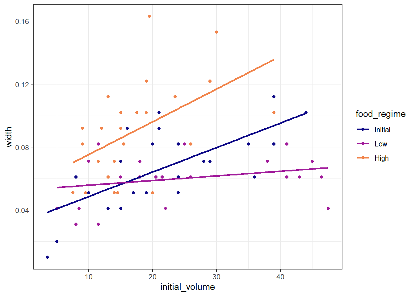
2.2 Building the Model
We start with a simple linear regression model using linear_reg(). The tidymodels ecosystem separates model specification (what model we want) from the computational engine (how it is estimated). The parsnip package handles this abstraction.
Available engines for linear_reg() are listed here: https://parsnip.tidymodels.org/reference/linear_reg.html
- Choose the model type:
linear_reg()Linear Regression Model Specification (regression)
Computational engine: lm - Choose the engine:
linear_reg() |>
  set_engine("lm")
Linear Regression Model Specification (regression)
Computational engine: lm - Save the model specification:
mdl_Linear <- linear_reg()2.3 Training (Fitting) the Model
To train the model, we use the fit() function, which requires:
- the model specification
- a formula
- the training dataset
fit_Linear <-
  mdl_Linear |>
  fit(width ~ initial_volume * food_regime, data = df_Urchins)

fit_Linear
parsnip model object
Call:
stats::lm(formula = width ~ initial_volume * food_regime, data = data)
Coefficients:
(Intercept) initial_volume
0.0331216 0.0015546
food_regimeLow food_regimeHigh
0.0197824 0.0214111
initial_volume:food_regimeLow initial_volume:food_regimeHigh
-0.0012594 0.0005254 We can inspect the fitted model coefficients:
tidy(fit_Linear)# A tibble: 6 × 5
term estimate std.error statistic p.value
<chr> <dbl> <dbl> <dbl> <dbl>
1 (Intercept) 0.0331 0.00962 3.44 0.00100
2 initial_volume 0.00155 0.000398 3.91 0.000222
3 food_regimeLow 0.0198 0.0130 1.52 0.133
4 food_regimeHigh 0.0214 0.0145 1.47 0.145
5 initial_volume:food_regimeLow -0.00126 0.000510 -2.47 0.0162
6 initial_volume:food_regimeHigh 0.000525 0.000702 0.748 0.457 2.4 Predicting with the Fitted Model
Once a model is fitted, we can use it for prediction. To make predictions we need:
- a dataset containing the feature variables (with matching names)
- the fitted model object
By default, predict() returns the mean prediction:
df_NewData <- expand.grid(
  initial_volume = 20,
  food_regime = c("Initial", "Low", "High")
)

pred_Mean <- predict(fit_Linear, new_data = df_NewData)
pred_Mean
# A tibble: 3 × 1
.pred
<dbl>
1 0.0642
2 0.0588
3 0.0961We can also request confidence intervals using type = "conf_int":
pred_Conf <- predict(
  fit_Linear,
  new_data = df_NewData,
  type = "conf_int"
)
pred_Conf
# A tibble: 3 × 2
.pred_lower .pred_upper
<dbl> <dbl>
1 0.0555 0.0729
2 0.0499 0.0678
3 0.0870 0.105 3 Data Processing with recipes
The recipes package provides a structured and extensible framework for data preprocessing and feature engineering within the tidymodels ecosystem.
It allows us to define all preprocessing steps in a reproducible, model-agnostic workflow before model fitting.
In this exercise, we will focus on the following steps:
- Data splitting – Dividing the dataset into training, validation, and testing sets.
- Recipe defining
2.1 Basic definition – Specifying the target variable, predictors, and initial preprocessing steps.
2.2 Feature engineering – Applying transformations, scaling, encoding, and other preprocessing techniques to enhance model performance.
- Model building – Selecting and configuring the appropriate algorithm for the task.
- Combining recipe and model into a workflow – Integrating preprocessing steps with the model into a unified pipeline.
- Model fitting – Training the model on the training data using the defined workflow.
- Prediction – Generating predictions on new or unseen data.
- Evaluation – Assessing model performance using suitable metrics and interpreting the results to inform potential improvements.
3.1 Data
In this example we work with flight information from the United States (package nycflights13).
Our goal is to predict whether an arriving flight is late (arrival delay ≥ 30 minutes) or on time.
The modeling relationship can be summarized as:
arr_delay ~ (date, airport, distance, ...)library(nycflights13)
set.seed(123)
df_Flight <-
flights |>
mutate(
arr_delay = ifelse(arr_delay >= 30, "late", "on_time"),
arr_delay = factor(arr_delay),
date = lubridate::as_date(time_hour)
) |>
inner_join(weather, by = c("origin", "time_hour")) |>
select(dep_time, flight, origin, dest, air_time, distance,
carrier, date, arr_delay, time_hour) |>
na.omit() |>
mutate_if(is.character, as.factor)
df_Flight |>
skimr::skim(dest, carrier)| Name | df_Flight |
| Number of rows | 325819 |
| Number of columns | 10 |
| _______________________ | |
| Column type frequency: | |
| factor | 2 |
| ________________________ | |
| Group variables | None |
Variable type: factor
| skim_variable | n_missing | complete_rate | ordered | n_unique | top_counts |
|---|---|---|---|---|---|
| dest | 0 | 1 | FALSE | 104 | ATL: 16771, ORD: 16507, LAX: 15942, BOS: 14948 |
| carrier | 0 | 1 | FALSE | 16 | UA: 57489, B6: 53715, EV: 50868, DL: 47465 |
3.2 Data Split
As usual, we divide the dataset into training and validation sets. This allows us to fit the model on one portion of the data and evaluate performance on unseen observations.
Under the tidymodels framework:
initial_split()performs the random split.training()andtesting()extract the corresponding sets.
set.seed(222)
split_Flight <- initial_split(df_Flight, prop = 3/4)

df_Train <- training(split_Flight)
df_Validate <- testing(split_Flight)
3.3 Creating a Recipe
3.3.1 Basical Recipe
A recipe in tidymodels is a structured, pre-defined plan for data preprocessing and feature engineering.
It allows us to declare, in advance, all the steps needed to transform raw data into model-ready features.
When creating a recipe, two fundamental components must be specified:
Formula (
~):
The variable on the left-hand side is the target/outcome, and the variables on the right-hand side are the predictors/features.Data:
The dataset is used to identify variable names and types. At this stage, no transformations are applied.
# Create a basic recipe
rcp_Flight <- recipe(arr_delay ~ ., data = df_Train)
Using . on the right-hand side indicates that all remaining variables in the dataset should be used as predictors.
3.3.2 Roles
In addition to the standard roles (outcome and predictor), recipes allows defining custom roles using update_role().
Common roles include:
predictor: variables used to predict the outcomeoutcome: target variableID: identifiers not used for modelingcase_weights: observation weightsdatetime,latitude,longitude: for temporal or spatial feature engineering
rcp_Flight <-
  recipe(arr_delay ~ ., data = df_Train) |>
  update_role(flight, time_hour, new_role = "ID")

summary(rcp_Flight)
# A tibble: 10 × 4
variable type role source
<chr> <list> <chr> <chr>
1 dep_time <chr [2]> predictor original
2 flight <chr [2]> ID original
3 origin <chr [3]> predictor original
4 dest <chr [3]> predictor original
5 air_time <chr [2]> predictor original
6 distance <chr [2]> predictor original
7 carrier <chr [3]> predictor original
8 date <chr [1]> predictor original
9 time_hour <chr [1]> ID original
10 arr_delay <chr [3]> outcome original3.4 Feature Engineering with step_*
3.4.1 Date Features
Feature engineering transforms raw data into model-ready variables. recipes expresses each transformation as a step_*() function.
Below, we extract:
- day of week (
dow) - month
- holiday indicators (using U.S. holidays)
rcp_Flight <-
  recipe(arr_delay ~ ., data = df_Train) |>
  update_role(flight, time_hour, new_role = "ID") |>
  step_date(date, features = c("dow", "month")) |>
  step_holiday(
    date,
    holidays = timeDate::listHolidays("US"),
    keep_original_cols = FALSE
  )
This replaces the original date with engineered calendar features.
3.4.2 Categorical Variables (Dummy Encoding)
Most models require converting categorical variables into dummy/one-hot encoded predictors. recipes provides:
step_novel(): handles unseen factor levels at prediction timestep_dummy(): converts categorical predictors into numerical dummy variables
rcp_Flight <-
  recipe(arr_delay ~ ., data = df_Train) |>
  update_role(flight, time_hour, new_role = "ID") |>
  step_date(date, features = c("dow", "month")) |>
  step_holiday(
    date,
    holidays = timeDate::listHolidays("US"),
    keep_original_cols = FALSE
  ) |>
  step_novel(all_nominal_predictors()) |>
  step_dummy(all_nominal_predictors())
3.4.3 Removing Zero-Variance Predictors
Predictors with constant values provide no information and may cause issues in some algorithms. We remove them using step_zv():
rcp_Flight <-
  recipe(arr_delay ~ ., data = df_Train) |>
  update_role(flight, time_hour, new_role = "ID") |>
  step_date(date, features = c("dow", "month")) |>
  step_holiday(
    date,
    holidays = timeDate::listHolidays("US"),
    keep_original_cols = FALSE
  ) |>
  step_novel(all_nominal_predictors()) |>
  step_dummy(all_nominal_predictors()) |>
  step_zv(all_predictors())
3.5 Combining the Recipe with a Model
3.5.1 Workflow Definition
In this section, we formalize the integration of data preprocessing and model specification by constructing a workflow. This approach ensures that all preprocessing operations defined in the recipe are applied consistently during model training and prediction, thereby maintaining a coherent pipeline.
A workflow allows bundling:
- the recipe (preprocessing)
- the model (statistical/ML algorithm)
mdl_LogReg <-
  logistic_reg() |>
  set_engine("glm")

wflow_Flight <-
  workflow() |>
  add_model(mdl_LogReg) |>
  add_recipe(rcp_Flight)
3.6 Model Fitting
We proceed by fitting the complete preprocessing and modeling pipeline to the training data using the fit() function.
fit_Flight <-
  wflow_Flight |>
  fit(data = df_Train)
Inspect model coefficients:
fit_Flight |>
  extract_fit_parsnip() |>
  tidy()
# A tibble: 157 × 5
term estimate std.error statistic p.value
<chr> <dbl> <dbl> <dbl> <dbl>
1 (Intercept) 7.28 2.73 2.67 7.64e- 3
2 dep_time -0.00166 0.0000141 -118. 0
3 air_time -0.0440 0.000563 -78.2 0
4 distance 0.00507 0.00150 3.38 7.32e- 4
5 date_USChristmasDay 1.33 0.177 7.49 6.93e-14
6 date_USColumbusDay 0.724 0.170 4.25 2.13e- 5
7 date_USCPulaskisBirthday 0.807 0.139 5.80 6.57e- 9
8 date_USDecorationMemorialDay 0.585 0.117 4.98 6.32e- 7
9 date_USElectionDay 0.948 0.190 4.98 6.25e- 7
10 date_USGoodFriday 1.25 0.167 7.45 9.40e-14
# ℹ 147 more rows3.7 Prediction
Upon fitting, the workflow is employed to generate predictions on the validation dataset.
pred_Flight <- predict(fit_Flight, df_Validate)For evaluation we need both class predictions and class probabilities:
pred_Flight <-
  predict(fit_Flight, df_Validate, type = "prob") |>
  bind_cols(predict(fit_Flight, df_Validate, type = "class")) |>
  bind_cols(df_Validate |> select(arr_delay))
3.8 Evaluation
The predictive performance of the model is evaluated using appropriate metrics, including ROC AUC and accuracy. Additionally, visualization of the ROC curve facilitates an assessment of the classifier’s discriminative capability.
pred_Flight |>
  roc_auc(truth = arr_delay, .pred_late)
# A tibble: 1 × 3
.metric .estimator .estimate
<chr> <chr> <dbl>
1 roc_auc binary 0.764pred_Flight |>
accuracy(truth = arr_delay, .pred_class)# A tibble: 1 × 3
.metric .estimator .estimate
<chr> <chr> <dbl>
1 accuracy binary 0.849aug_Flight <- augment(fit_Flight, df_Validate)
aug_Flight |>
roc_curve(truth = arr_delay, .pred_late) |>
autoplot()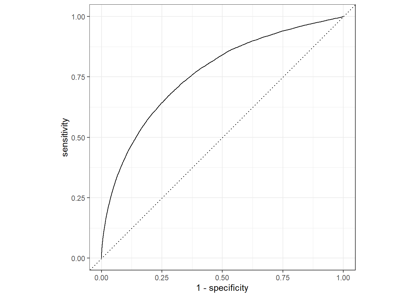
3.9 Clean Version of the Code
set.seed(222) # Set seed for reproducibility
# Split the data into 75% training and 25% validation
split_Flight <- initial_split(df_Flight, prop = 3/4)
df_Train <- training(split_Flight) # Extract training set
df_Validate <- testing(split_Flight) # Extract validation set
# -------------------------------
# Create a preprocessing recipe
# -------------------------------
rcp_Flight <-
recipe(arr_delay ~ ., data = df_Train) |> # Define target and predictors
update_role(flight, time_hour, new_role = "ID") |> # Assign ID role to identifier columns
step_date(date, features = c("dow", "month")) |> # Extract day of week & month from date
step_holiday(
date,
holidays = timeDate::listHolidays("US"),
keep_original_cols = FALSE
) |> # Add holiday indicator features
step_novel(all_nominal_predictors()) |> # Handle new factor levels in prediction
step_dummy(all_nominal_predictors()) |> # Convert categorical predictors to dummy variables
step_zv(all_predictors()) # Remove predictors with zero variance
# -------------------------------
# Define the logistic regression model
# -------------------------------
mdl_LogReg <-
logistic_reg() |>
set_engine("glm") # Use generalized linear model as backend
# -------------------------------
# Combine recipe and model into a workflow
# -------------------------------
wflow_Flight <-
workflow() |>
add_model(mdl_LogReg) |>
add_recipe(rcp_Flight)
# -------------------------------
# Fit the workflow on the training data
# -------------------------------
fit_Flight <-
wflow_Flight |>
fit(data = df_Train)
# -------------------------------
# Predict on the validation set (class labels)
# -------------------------------
pred_Flight <- predict(fit_Flight, df_Validate)
# -------------------------------
# Predict on validation set (probabilities and class labels)
# -------------------------------
pred_Flight <-
predict(fit_Flight, df_Validate, type = "prob") |> # Predicted probabilities
bind_cols(predict(fit_Flight, df_Validate, type = "class")) |> # Predicted classes
bind_cols(df_Validate |> select(arr_delay)) # Add true labels for evaluation
# -------------------------------
# Evaluate model performance
# -------------------------------
pred_Flight |>
roc_auc(truth = arr_delay, .pred_late) # ROC AUC for "late" class
pred_Flight |>
  accuracy(truth = arr_delay, .pred_class)
# Classification accuracy
# -------------------------------
# Visualize ROC curve
# -------------------------------
aug_Flight <- augment(fit_Flight, df_Validate) # Add predictions and residuals to dataset
aug_Flight |>
roc_curve(truth = arr_delay, .pred_late) |> # Compute ROC curve
autoplot() # Plot ROC curve4 Modelling with Resampling
In contrast to the previous exercise, this section introduces model evaluation using resampling techniques, specifically cross-validation. This approach incorporates an additional step in which the training dataset is repeatedly partitioned into multiple training–validation splits. By fitting and evaluating the model across these resampled subsets, cross-validation provides a more reliable and robust estimate of the model’s generalization performance than a single train–validate split.
4.1 Evaluating Training and Validation Sets
A fitted model can be evaluated on both the training dataset and the validation (test) dataset.
After generating predictions, we can compute performance metrics such as roc_auc and accuracy.
For both metrics, higher values indicate better predictive performance.
library(modeldata)

# ----------------------------------
# Dataset
# ----------------------------------

## Split the data
set.seed(123)
split_Cell <- initial_split(
  modeldata::cells |> select(-case),
  strata = class
)

df_Train_Cell <- training(split_Cell)
df_Validate_Cell  <- testing(split_Cell)

# ----------------------------------
# Model
# ----------------------------------

## Specify a random forest classifier
mdl_RandomForest <-
  rand_forest(trees = 1000) |>
  set_engine("ranger") |>
  set_mode("classification")

## Fit the model
set.seed(234)
fit_RandomForest <-
  mdl_RandomForest |>
  fit(class ~ ., data = df_Train_Cell)
fit_RandomForest
parsnip model object
Ranger result
Call:
ranger::ranger(x = maybe_data_frame(x), y = y, num.trees = ~1000, num.threads = 1, verbose = FALSE, seed = sample.int(10^5, 1), probability = TRUE)
Type: Probability estimation
Number of trees: 1000
Sample size: 1514
Number of independent variables: 56
Mtry: 7
Target node size: 10
Variable importance mode: none
Splitrule: gini
OOB prediction error (Brier s.): 0.1187479 # ----------------------------------
# Predictions
# ----------------------------------
## Training set predictions
pred_Train_Cell <-
predict(fit_RandomForest, df_Train_Cell) |>
bind_cols(predict(fit_RandomForest, df_Train_Cell, type = "prob")) |>
bind_cols(df_Train_Cell |> select(class))
## Validation set predictions
pred_Validate_Cell <-
predict(fit_RandomForest, df_Validate_Cell) |>
bind_cols(predict(fit_RandomForest, df_Validate_Cell, type = "prob")) |>
bind_cols(df_Validate_Cell |> select(class))
# ----------------------------------
# Performance
# ----------------------------------
## Training
pred_Train_Cell |> roc_auc(truth = class, .pred_PS)# A tibble: 1 × 3
.metric .estimator .estimate
<chr> <chr> <dbl>
1 roc_auc binary 1.000pred_Train_Cell |> accuracy(truth = class, .pred_class)# A tibble: 1 × 3
.metric .estimator .estimate
<chr> <chr> <dbl>
1 accuracy binary 0.990## Validation
pred_Validate_Cell |> roc_auc(truth = class, .pred_PS)# A tibble: 1 × 3
.metric .estimator .estimate
<chr> <chr> <dbl>
1 roc_auc binary 0.891pred_Validate_Cell |> accuracy(truth = class, .pred_class)# A tibble: 1 × 3
.metric .estimator .estimate
<chr> <chr> <dbl>
1 accuracy binary 0.814The results typically show a large gap between training and validation performance. This is normal: the model tends to overfit the training data, leading to reduced predictive ability on new, unseen data. This is precisely why a simple train/test split is often insufficient. To obtain more reliable and stable performance estimates, we use resampling methods.
4.2 Resampling (Cross-Validation)
Cross-validation improves model evaluation by repeatedly splitting the training data into several folds. Each fold is used once as an assessment (test) set, while the remaining folds form the analysis (training) set.
This process reduces the variance in performance estimation and helps detect overfitting.
set.seed(345)
folds_Cell <- vfold_cv(df_Train_Cell, v = 10)

wflow_CrossValidate <-
  workflow() |>
  add_model(mdl_RandomForest) |>
  add_formula(class ~ .)

set.seed(456)
fit_CrossValidate <-
  wflow_CrossValidate |>
  fit_resamples(folds_Cell)

collect_metrics(fit_CrossValidate)
# A tibble: 3 × 6
.metric .estimator mean n std_err .config
<chr> <chr> <dbl> <int> <dbl> <chr>
1 accuracy binary 0.833 10 0.00876 Preprocessor1_Model1
2 brier_class binary 0.120 10 0.00406 Preprocessor1_Model1
3 roc_auc binary 0.905 10 0.00627 Preprocessor1_Model1Compared with normal model fitting, resampling uses the specialized function:
fit_resamples()which fits the model on each fold and aggregates the performance results.
Cross-validation therefore provides a more robust estimate of the model’s generalization ability and reduces the risk of overfitting, compared with a single train/test split.